V Plotter Design

A V plotter is a minimalistic design which uses a pair of steppers, some string, and a pen head to create a plotter. These are sometimes made by students or technology sector employees as a way to avoid "real work".

In this article, I dig into the math behind these machines, and also write a program to calculate the configuration of a V setup needed to produce a working device.

Requirements

What is the optimal configuration of control lines for an area to be plotted? Obviously, we can't have a drawing area above the control lines — our friend gravity sees to that. But, can we do better than hand waving and "somewhere below the control lines" for the plot area? Yes: we think up some constraints and model them with math and code (two more friends!):

Tension: We can imagine that the control lines have to be under some tension in order to be effective. For the purposes of this article we say that both string tensions must be in the range [ m/2, m*1.5 ], where m is the mass of the plotter head. Lines can neither be too slack nor too heavily loaded. The effect of this constraint is to prevent any line from being too close to horizontal or too close to vertical.
Resolution: There is a change in resolution when we map a change of length in one or both of the strings into X and Y coordinates. I.e. Coordinate system conversion causes a non-uniform step resolution. We say that, for each control line, a one unit change causes at most a 1.4 unit change in the X,Y coordinate system. We limit plotting to the area of reasonable resolution. Here our definition of reasonable is a 40% change.

To implement these requirements, we need to know how to calculate them. The next few sections talk math and have pretty pictures.

Line Tension Calculation

The below diagram shows a mass m suspended by two lines. Each line can (and usually will) have a different angle to the X axis. We wish to calculate the tension of each line in the diagram.

V plotter force vectors

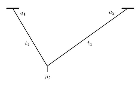
To describe the horizontal forces along the X axis (in balance), we write:

$t_{1}\cdot\cos a_{1}=t_{2}\cdot\cos a_{2}$

To describe the force m along the Y axis, caused by the weight of the plotter head assembly, we write:

$t_{1}\cdot\sin a_{1}+t_{2}\cdot\sin a_{2}=m$

Solving these two equations in terms of tension, we get:

$t_{1}=\frac{\cos a_{2} \cdot m} {\cos a_{1} \cdot \sin a_{2} + \sin a_{1} \cdot \cos a_{2}}$

and

$t_{2}=\frac{\cos a_{1} \cdot m} {\cos a_{1} \cdot \sin a_{2} + \sin a_{1} \cdot \cos a_{2}}$

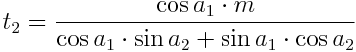
Note that the tension equations have denominators in common.

Angle Length Cartesian Conversion

We wish to translate between coordinate systems:

From an angle and a length (here based from the origin), we wish to find an X,Y coordinate.
From an X,Y coordinate pair, we wish to find the angle and length (here to the origin).

This is visualized below.

coordinate system conversion

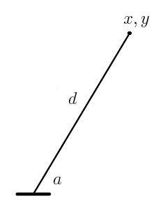
Trigonometry tells us that:

$x,y = \cos a \cdot d, \sin a \cdot d$

$d,a = \sqrt{x^2+y^2}, \mathrm{atan2}(y,x)$

See Wikipedia article on atan2. Adjusting these formulas for non-origin locations involves a simple addition or subtraction adjustment.

I don't think there is a name for the coordinate system using two control lines. The closest I can find is the biangular coordinate system, but this has more to do with the angles of the lines to the X axis than the length of the lines. As long as I am in confession mode, I must also say that I have not seen "V plotter" being used as the name of this kind of device. I am not able to find any established name for this "thing", so necessity became the mother of invention.

Law of Cosines

The law of cosines can be used for many applications, here we use it to find an angle when we know the length of three legs.

law of cosines triangle

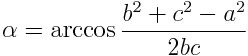
The law of cosines allows us to calculate the position of the print head when a line changes length. The basic form of the law is:

$a^2=b^2+c^2-2bc\cos\alpha$

Solving for α (alpha) we get:

$\alpha = \arccos\frac{b^2+c^2-a^2}{2bc}$

The code uses this to map where the resolution of the print head is within an acceptable range. At certain points, a small change in line length will result in too large a change in the x,y coordinate system.

To check for resolution, we adjust a or b, then use the law of cosines to find α (alpha). Knowing α (alpha), length b and position A, we can use simple sine and cosine (see previous section) to find position C.

Code Simulation

Now we have enough math to code a V plotter simulation. The code below is divided into sections, each section is introduced with information to know when reading the the code itself. The code sections can be pasted together to produce a complete Python program to run the simulation and draw the plotting area.

First we reference some libraries and set some constants.

#!/usr/bin/env python
import sys,Image,ImageDraw
from math import sqrt,sin,cos,acos,atan2,degrees,fabs
# setup the constants
version=1.7
outputFile="out.png"
width,height=800,600
border=32
# V line end points
v1=border/2,border/2
v2=width-border/2-1,border/2

Here we draw the fixed parts of the picture: the crosses showing the end points of the control lines, and the background for the drawing. Note that this drawing package has the origin in the upper left hand corner and a Y axis with positive values progressing downward.

def cross(draw,p,n):
    c="#000000"
    draw.line((p[0],p[1]-n,p[0],p[1]+n),c)
    draw.line((p[0]-n,p[1],p[0]+n,p[1]),c)

def drawFixtures(draw):
    # border of calculation pixels
    draw.rectangle([border-1,border-1,width-border,height-border],"#FFFFFF","#000000")
    # V line end points
    cross(draw,v1,border/4)
    cross(draw,v2,border/4)

There is a one to one correspondence between the tension calculation code here and the tension calculation derivation in the first math section.

def lineTensions(a1,a2):
    d=cos(a1)*sin(a2)+sin(a1)*cos(a2)
    return cos(a2)/d,cos(a1)/d

def tensionOk(p):
    # find angles
    a1=atan2(p[1]-v1[1],p[0]-v1[0])
    a2=atan2(p[1]-v2[1],v2[0]-p[0])
    # strings tension check
    t1,t2=lineTensions(a1,a2)
    lo,hi=.5,1.5
    return lo<t1<hi and lo<t2<hi

Similarly, the resolution check code here is an implementation of the math in the previous section. In addition, there is a "sanity check" to verify that the calculated point for the triangle is the same as the point passed in to the calculation.

def dx(p1,p2):
    return sqrt((p1[0]-p2[0])**2+(p1[1]-p2[1])**2);

def calcPointB(a,b,c):
    alpha=acos((b**2+c**2-a**2)/(2*b*c))
    return b*cos(alpha)+v1[0],b*sin(alpha)+v1[1]

def resolutionOk(p):
    max=1.4
    # law of cosines calculation and nomenclature
    c=dx(v1,v2)
    b=dx(v1,p)
    a=dx(v2,p)
    # sanity check
    err=.00000000001
    pc=calcPointB(a,b,c)
    assert p[0]-err<pc[0]<p[0]+err
    assert p[1]-err<pc[1]<p[1]+err
    # calculate mapped differences
    db=dx(p,calcPointB(a,b+1,c)) # extend left line by 1 unit
    da=dx(p,calcPointB(a+1,b,c)) # extend right line by 1 unit
    return db<max and da<max # line pull of 1 unit does not move x,y by more than max

Each pixel in the drawing area is assigned a color based on the tension and resolution calculations. Dots are written on the terminal window to indicate that the calculation is underway.

def calcPixel(draw,p):
    t=tensionOk(p)
    r=resolutionOk(p)
    if not t and not r:
        draw.point(p,"#3A5FBD")
    if not t and r:
        draw.point(p,"#4876FF")
    if t and not r:
        draw.point(p,"#FF7F24")
    # default to background color

def drawPixels(draw):
    for y in range(border,height-border):
        sys.stdout.write('.')
        sys.stdout.flush()
        for x in range(border,width-border):
            calcPixel(draw,(x,y))
    sys.stdout.write('\n')

The main section of the program prepares an image for the calculation and writes it to disk when done.

def main():
    print "V plotter map, version", version

    image = Image.new("RGB",(width,height),"#D0D0D0")
    draw = ImageDraw.Draw(image)

    drawFixtures(draw)
    drawPixels(draw)

    image.save(outputFile,"PNG")
    print "map image written to", outputFile
    print "done."

if __name__ == "__main__":
    main()

To read code "top down" (more general to more detailed), start reading at the bottom section and work your way up. Oops, it's too late for me to tell you that now. Sorry.

Plot Area Map

The output of the program is a picture mapping locations to how well they met the specified requirements.

V plotter design Map

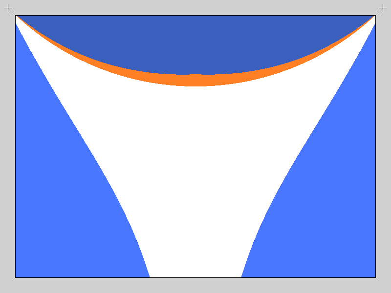
Colors designate:

Orange: poor resolution
Light Blue: too little tension in one of the lines
Dark Blue: too much tension in one of the lines (and poor resolution)
White: drawing area candidate

It is interesting to see that the area with poor resolution is a superset (entirely covers) the area with too much line tension. Thinking about it makes some intuitive sense: this is similar to a lever with a heavy weight on the short arm making the long arm move up or down a greater distance.

We see light blue sections under each "+" line control point. This also makes some intuitive sense because supporting a weight with a vertical line leaves no work (or tension) for an adjacent line. The light blue area on each side shows the loss of line tension on the side opposite. This is unfortunate because there is also line sag in longer lines (not covered in the above math or simulation) which is exacerbated by the loss of tension.

Given V plotter control lines sourced at the "+" markers, reasonable plotting can be done in the white region. For square or rectangular physical plotting surface, we can make a panel with the top side touching the orange area and the bottom corners touching the light blue area. For example the green area in the picture below:

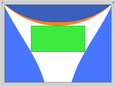
drawing surface in V plotter design Map

The ends of the control lines in the above picture seem to be further away from the plotting surface than V plotters commonly seen on the internet. Specifying different constraints will give different possibilities for drawing areas. We now have the tools in hand to parametrically design a V plotter matching the constraints we desire.